Portfolite – Framer Portfolio Template

Dibs E-Commerce Data Analytics & Sales Forecasting

Objective

to analyse historical data for Dibs, an online tech retailer facing declining sales and customer retention issues. Through data wrangling, deep analysis, and time-series modelling, the project aimed to uncover patterns in customer purchasing behaviour, geographic performance, and temporal sales trends. The ultimate goal was to deliver data-driven recommendations to optimise marketing strategies, improve product bundling, and drive revenue growth.

tool

R, tidyverse, ggplot2, forecast, keras (LSTM), ARIMA, Time-Series Analysis, Neural Networks

firm analysed

dibs

Role

Data Analyst

PROJECT OVERVIEW

Dibs, a rising online technological retail company in the US, faced stagnating sales and customer retention challenges following the abrupt impacts of the COVID-19 pandemic. The objective of this project was to leverage a highly complex, raw dataset of historical sales to extract actionable insights.

My specific contribution focused on transforming cleansed data into strategic business value. I led the deep analysis of purchasing patterns, engineered advanced data visualisations to map operational trends, and deployed machine learning models to forecast future sales, ultimately delivering targeted, data-driven marketing and operational recommendations.

KEY FINDINGS

1. The Revenue Anchor

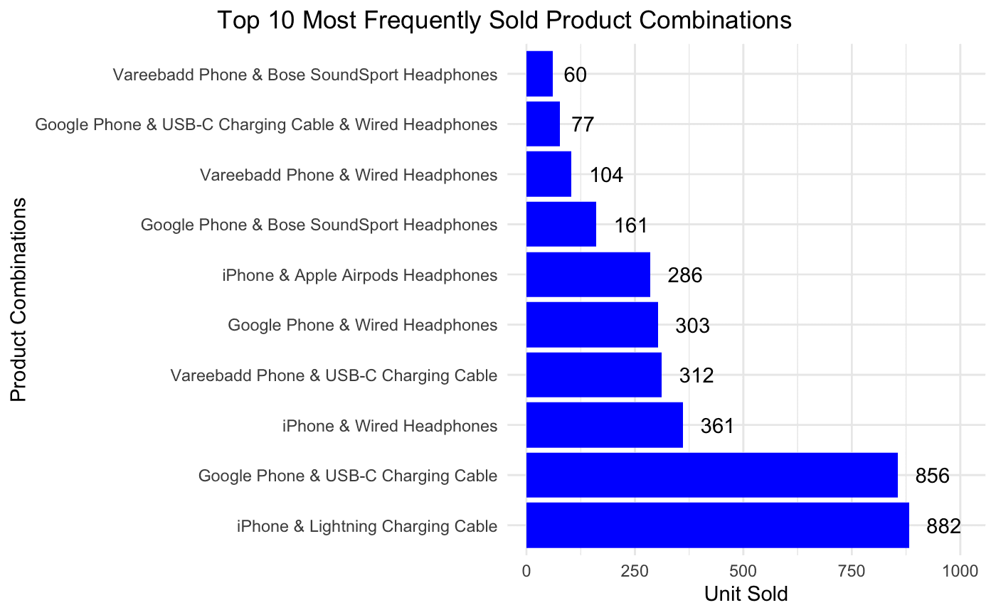
Understanding what customers buy together is crucial for cross-selling and bundling strategies. I conducted an in-depth analysis of frequently grouped products by isolating unique Order.ID values to identify items purchased in the same transaction.

A key finding was the high frequency of mobile phones being bought alongside charging cables rather than headphones. This insight directly informed our bundling strategies, reflecting the modern tech landscape where manufacturers no longer include adapters in the box.

#Find the unique values of product and allign them with product category column:
unique(df3$Product)
# Find duplicated Order.IDs
duplicated_orders <- df3 %>%
  group_by(Order.ID) %>%
  filter(n() > 1) %>%
#Create a total.product that take those product that having the same Order.ID
  summarise(total.product = paste(Product, collapse = " & "))

#Plot the frequencies of products that often being bought toghether

# Count the frequencies of total.product
product_frequencies <- duplicated_orders %>%
  count(total.product) %>%
  arrange(desc(n))

# Print the new data frame with frequencies
print(product_frequencies)

# Print the top 10 most frequent product combinations
top_10_product_combinations <- head(product_frequencies, 10)

# Visualize the top 10 most frequent product combinations
ggplot(top_10_product_combinations, aes(x = reorder(total.product, -n), y = n)) +
  geom_bar(stat = "identity", fill = "blue") +
  geom_text(aes(label = n), hjust = -0.5, color = "black") +
  coord_flip() +
  scale_y_continuous(expand = expansion(mult = c(0.05, 0.2))) + 
  labs(title = "Top 10 Most Frequently Sold Product Combinations",
       x = "Product Combinations",
       y = "Unit Sold") +
  theme_minimal() +
  theme(plot.title = element_text(hjust = 3))

# Extract hour from 'Order.Time' using word() function
Daily_Sale_2019 <- Daily_Sale_2019 %>%
  mutate(Hour = as.numeric(word(Order.Time, 1, sep = ":")))

# Summarize the total quantity ordered for each hour
hourly_order_trend <- Daily_Sale_2019 %>%
  group_by(Hour) %>%
  summarise(total_orders = round(sum(Quantity.Ordered, na.rm = TRUE))) %>%
  ungroup()

# Calculate the hourly average order
hourly_avg_order <- round(mean(hourly_order_trend$total_orders))

# Create a line graph illustrating Hourly order trend vs hourly average order
ggplot(hourly_order_trend, aes(x = Hour, y = total_orders)) +
  geom_line(color = "blue", size = 1) +  # Line for the hourly order trend
  geom_point(color = "blue", size = 2) +  # Points for hourly orders
  geom_hline(yintercept = hourly_avg_order, color = "red", linetype = "dashed", size = 1) +  # Horizontal line for hourly average
  labs(title = "Hourly Order Trend vs Hourly Average Order (2019 Total Order by Each Hour)",
       x = "Hour of the Day",
       y = "Whole Year Total Orders by Hour") +
  scale_x_continuous(breaks = 0:23) +  # Ensure full list of hours is shown
  scale_y_continuous(expand = expansion(mult = c(0.05, 0.1))) +  # Slightly extend y-axis
  theme_minimal() +
  theme(axis.text.x = element_text(angle = 45, hjust = 1, vjust = 1),
        plot.title = element_text(hjust = 0.5)) +
  annotate("text", x = 23, y = hourly_avg_order, 
           label = paste("Average Orders:", hourly_avg_order), 
           color = "red", vjust = -0.5, hjust = 4.1) +
  geom_text(data = hourly_order_trend %>% filter(Hour %in% c(3, 12, 15, 19)),
            aes(label = total_orders), 
            vjust = -1, color = "black", size = 3.5)

2. Visualising Business Operations

To optimise marketing spend and operational efficiency, it was necessary to map the business's natural traffic flow. I utilised ggplot2 to visualise sales trends across months, days, and hours.

The hourly order trend analysis revealed that order volumes consistently rise throughout the morning, experiencing a midday peak at 12:00 PM (14,202 orders), followed by the absolute peak of the trading cycle at 7:00 PM (14,470 orders). This data is invaluable for timing digital ad campaigns and scheduling server maintenance.

3. Predictive Modelling: Time-Series Forecasting

To predict future sales trajectories, I implemented and compared two distinct time-series forecasting models using an 80/20 train-test split:

ARIMA: A classical statistical method effective for linear patterns.
LSTM (Long Short-Term Memory Neural Network): An advanced deep learning model highly effective at capturing complex, non-linear temporal dependencies, built using keras.

Model Evaluation: The LSTM model significantly outperformed the ARIMA model, achieving a much lower Root Mean Squared Error (RMSE of 17,537 vs. 22,492). Consequently, I deployed the LSTM model to forecast the next 30 days of daily sales for January 2020.

Baseline Forecasting - ARIMA

The Autoregressive Integrated Moving Average (ARIMA) model was selected as a robust baseline statistical method to identify and forecast linear patterns and seasonality within the sales data .

While the model successfully mapped the general upward trend of late 2019, it struggled to precisely capture the sharp, complex daily fluctuations during peak holiday periods, returning a Root Mean Squared Error (RMSE) of 22,492 on the test data.

# Define the split date for training and testing (train:test = 8:2)
split_date <- as.Date("2019-10-19") 

# Split the data into training and test sets
train_ts <- window(ts_sales, end = c(year(split_date), yday(split_date) - 1))
test_ts <- window(ts_sales, start = c(year(split_date), yday(split_date)))

# Print the training and test sets
print(train_ts)
print(test_ts)

# Build the ARIMA model
fit_arima <- auto.arima(train_ts)

# Print the model summary
summary(fit_arima)

# Forecast the next month using ARIMA
forecast_arima <- forecast(fit_arima, h = length(test_ts))

# Print the forecast
print(forecast_arima)

# Plot the forecast
autoplot(forecast_arima) + autolayer(test_ts, series = "Actual")

# Calculate the accuracy
accuracy(forecast_arima, test_ts)

Advanced Forecasting - LSTM

To capture the intricate, non-linear behaviours present in the daily sales fluctuations, I deployed a Long Short-Term Memory (LSTM) recurrent neural network .

The LSTM model significantly outperformed the baseline ARIMA model. By effectively learning long-term dependencies in the sequence data, the LSTM model achieved a much tighter fit to the actual testing data, lowering the RMSE to 17,537.

# Function to create sequences for the neural network
create_sequences <- function(data, seq_length) {
  x <- array(dim = c(length(data) - seq_length, seq_length, 1))
  y <- array(dim = c(length(data) - seq_length, 1))
  for (i in seq_len(length(data) - seq_length)) {
    x[i,,] <- data[i:(i + seq_length - 1)]
    y[i,] <- data[i + seq_length]
  }
  list(x = x, y = y)
}

SEQ_LENGTH <- 15 
train_sequences <- create_sequences(train_ts, SEQ_LENGTH)
x_train <- train_sequences$x
y_train <- train_sequences$y

# Define the LSTM model architecture
model <- keras_model_sequential() %>%
  layer_lstm(units = 60, return_sequences = TRUE, input_shape = c(SEQ_LENGTH, 1)) %>%
  layer_lstm(units = 60) %>%
  layer_dense(units = 1)

model %>% compile(
  loss = 'mean_squared_error',
  optimizer = optimizer_adam()
)

# Train the model
history <- model %>% fit(
  x_train, y_train,
  epochs = 100,
  batch_size = 32,
  validation_split = 0.2
)

Future Projection: January 2020 Sales Forecast

Given the LSTM model's superior predictive accuracy, I utilised it to generate a 30-day sales forecast for January 2020.

The forecast revealed a distinct post-holiday downward trend, predicting that daily revenue would decline and stabilise around $117,269 by the end of January. This critical insight allowed me to recommend that Dibs adjust their immediate inventory procurement and prepare targeted promotional campaigns to mitigate the anticipated seasonal slump.

# Predict the next 30 days iteratively
future_steps <- 30
last_sequence <- scaled_data[(length(scaled_data) - SEQ_LENGTH + 5):length(scaled_data)]
future_predictions <- numeric(future_steps)

for (i in 1:future_steps) {
  input_sequence <- array(last_sequence, dim = c(1, SEQ_LENGTH, 1))
  next_prediction <- model %>% predict(input_sequence)
  future_predictions[i] <- as.numeric(next_prediction)
  last_sequence <- c(last_sequence[-1], next_prediction)
}

# Inverse scale the future predictions back to actual dollar values
center <- scaler$mean
scale <- scaler$std
future_predictions <- future_predictions * scale + center

# Plot the future predictions
plot(daily_sales$Order.Date, daily_sales$daily_sales, type = 'l', col = 'blue', 
     xlab = 'Date', ylab = 'Sales', xlim = c(min(daily_sales$Order.Date), max(future_dates)+3))
lines(future_dates, future_predictions, col = 'red')
title(main = "Sales Forecast for January 2020")